Instead of reading about dead zones — set them yourself. The simulator starts with a demo link (two closely spaced connectors, a splice, a bend, a fiber end), but you can build your own: add connectors, splices, bends and splitters, drag them across the chart and watch the trace recompute live.
hover = measure · click a ▲ marker = edit event · drag a marker = move event · scroll wheel = zoom · drag background = pan view
The longer the pulse, the larger the dead zone and the higher the backscatter level — but also the greater the dynamic range. This is the fundamental trade-off of every OTDR measurement.
What you see on the trace
The falling line is Rayleigh backscatter — one millionth of the launched light returns to the detector, providing the “background” from which we read loss. The sharp peaks are Fresnel reflections at connectors and at the fiber end (the glass–air refractive-index step reflects up to 4% of the power). Downward steps with no reflection are splices and bends.
Dead zone and resolution
With a short pulse (100 ns), two connectors 60 m apart show up as separate events. Stretch the pulse to 1 µs and they merge into one — that is the event dead zone. At the same time, notice how the noise at the far end grows with a short pulse: less energy means less dynamic range, i.e. a shorter measurable link.
An important distinction: the physical pulse length in the fiber is about τ[ns]/10 meters (e.g. 100 ns ≈ 10 m). The event dead zone, however, is always somewhat larger — add the photodiode recovery time after saturation by a strong reflection, which for short pulses can be several times longer than the pulse itself. That is why the simulator shows both values separately. And if the dead zone at the start is suspiciously long despite a short pulse — first check the cleanliness of the OTDR port (chapter 6).
Launch and receive fibers
The OTDR port and the first connector generate a strong reflection and a dead zone — without a launch fiber the first connector of the link is unmeasurable: it merges with the port reflection and there is no backscatter in front of it from which its loss could be read. The launch fiber moves the link away from the port: the OTDR sees backscatter before and after the first connector of the link, so it can measure its loss and reflectance. The receive fiber does the same for the last connector — without it the end of the link is just a Fresnel peak dropping into the noise.
The handbook's rules: launch fiber length 1000–2000 m (a 20 µs pulse occupies as much as 2000 m of fiber — too short a launch fiber will merge the reflections again), fiber of the same type as the link (otherwise you buy yourself a gainer at the junction — see below), high-quality connectors. And the iron rule: connect the launch fiber directly to the link, with no intermediate patch cords — every extra junction is an event 1–2 m from the first connector of the link, i.e. inside its dead zone: the measurement is lost again, and an unknown loss sits in the path. See both scenarios in the event catalog below (the “Launch and receive fibers” card).
Ghosts
Turn on the “ghost”: when there are two strong reflections in the path (here the start connector and the connector at ~1 km), the pulse bounces back and forth between them. That extra path makes the reflectometer draw a false reflection — a peak like any other — at a distance equal to the spacing of those two reflections, repeated beyond the second one. You can recognize a ghost by its zero insertion loss: the trace after it does not drop by a single dB.
Splice loss: two-point or LSA (5-marker)?
The same splice loss of 0.20 dB on a noisy trace. The two-point method subtracts two single samples just before and just after the splice — and every sample carries noise, so each draw gives a different result. The LSA method (least squares approximation) fits regression lines to dozens of samples on both sides of the event and extrapolates them to its center (the dashed tails) — the vertical distance between the lines is the loss, and the noise averages out. That is why the OTDR screenshots in the handbook (Fig. 18, 29, 38) show “LSA” in the status bar. Redraw the noise a few times and compare the spreads:
the same 0.20 dB splice loss, the same readout positions — only the method differs
This is exactly the 5-marker (LSA) measurement from the reflectometer: markers ②–① set the window of the left line, ④–⑤ the window of the right one, and ③ sits on the event to which both lines are extrapolated. The same principle works for the attenuation of a section (dB/km) — LSA on a homogeneous segment instead of two points. One trap: the regression windows must be clean — if another event falls into them, the line will “smear” its loss and the result will lie.
Where the splices LSA can barely find come from
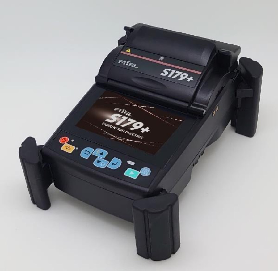
The FITEL S179+ aligns fibers to the core (core alignment): cameras analyze the position of the cores themselves and bring them together, pushing splice loss down to ~0.02 dB. These are events at the edge of detectability — which is why they are measured with the LSA method, not two points.
See it in the INTERLAB catalog →How far will my OTDR reach?
A practical rule: L ≈ (D − 6 dB − Σ event losses) / α. The ~6 dB margin above the noise floor is no whim — it is almost exactly the handbook's difference between the dynamic range specified for SNR=1 and the effective 0.1 dB dynamic range (6.6 dB, section 5.2.3): right at the noise floor you can still “see” the trace, but you can no longer measure attenuation reliably. Remember too that manufacturers specify dynamic range for the longest pulse and ~3 minutes of averaging.
A “512 km distance range” in the datasheet is only the maximum setting of the distance axis. How far you can really measure is determined solely by the dynamic range.
Hence two practical consequences. Long links: at 1310 nm the fiber alone eats ~0.35 dB/km — a 100 km link is ~34 dB, practically the entire dynamic range of a good field instrument; the same span at 1550 nm is ~20 dB. That is why long routes are measured with the 1550 + 1625 nm pair (both “make it”, and the loss difference still betrays bends), not 1310/1550. Splitters: a 1×32 is ~18 dB one way — and here high dynamic range buys something more valuable than kilometers: it lets you get through the splitter with the shortest possible pulse, and beyond the splitter the subscriber sections lie close together and only a short pulse will resolve them.
Before you press START
Four settings that are easy to forget: 1) measurement mode — real-time for a quick look and splicing checks, automatic for periodic measurements of known links, manual analysis where the automation gets lost; 2) distance range — set to about 2× the link length (too tight a range = wrapped-around ghosts, too wide = fewer points on the link); 3) index of refraction (IOR) — from the fiber manufacturer or determined on a section of known length; without it, distances lie; 4) fiber length ≠ cable length — fibers in loose tubes carry fiber overlength (the helix factor), so when locating a fault in the field, convert fiber meters to route meters using the cable data.
How much can you trust the result — accuracy and resolution
Start with the datasheet: manufacturers specify dynamic range using three different definitions (Fig. 27 of the handbook). D(SNR=1) — the IEC definition, down to the noise level; D(98%) — down to the level below which 98% of the noise samples lie; D(0.1 dB) — the effective range within which noise reaches 0.1 dB and a weak splice can still be measured reliably. The difference between D(SNR=1) and D(0.1 dB) is about 6.6 dB — a “30 dB” reflectometer measures 0.1 dB events only down to ~23.4 dB. That is exactly the margin the reach calculator above subtracts. (You will also come across RMS dynamic range: the IEC value minus 1.56 dB.)
The second axis — distance. The IEC 61746-1 standard breaks the location error into three components: scale error (the SL coefficient — in practice almost entirely a wrongly entered IOR: an error of 0.001 at n≈1.468 is ~0.7 m per kilometer, so at 10 km an event “shifts” by ~7 m), zero offset ΔL₀ (the position of the connector on the instrument panel) and sampling error — periodic, with an amplitude equal to the spacing of the measurement points; that is why, when locating a fault, it pays to densify the sampling (a shorter range, more points — good instruments go down to 5 cm).
The third — the power scale: dB reading accuracy rests on the linearity of the receiver chain (resolution ~0.01 dB). That is why in chapter 6 you measure an internal reference: the control chart catches drift of exactly this scale before it ruins your test reports.
Event catalog — how to recognize them on the trace
Every event in the path has its own “signature”. Reading these signatures is half of a technician's job — the other half is knowing when a signature can mislead. Click show and the simulator sets up a ready-made scenario.
Splice
A clean downward step in the backscatter, with no reflection peak — a splice creates no boundary between media. A good splice is 0.02–0.1 dB. Note: when joining different fibers, “gainers” appear — only a bidirectional measurement gives the true loss.
PC vs APC connector
A connector is loss plus a reflection peak. PC reflects about −45 dB. APC (ferrule polished at 8–9°) throws the reflection into the cladding: ≤ −60 dB. The peak height depends on reflectance relative to the backscatter, and backscatter grows with the pulse — which is why the APC peak disappears at 1 µs and re-emerges at 10 ns.
Bend (macrobend)
Loss without reflection — like a splice. How to tell them apart? Compare wavelengths: bend loss grows strongly with wavelength (1625 > 1550 ≫ 1310), while splice loss practically does not. That is why the handbook recommends measuring at two widely spaced wavelengths (Fig. 34).
Splitter
A big step: 1×2 ≈ 3.5 dB, 1×4 ≈ 6.9 dB, 1×8 ≈ 9.8 dB (Table 6). A PLC splitter is practically non-reflective. Beyond the splitter the signal often drowns in the noise — the dynamic range runs out.
Fiber end
A strong Fresnel reflection — the glass–air boundary reflects up to 4% of the power (about −14 dB) — followed by a cliff into the noise. No peak at the end? The fiber may be submerged, crushed, or terminated with an APC connector.
Ghost
A false peak from multiple reflection between two strong reflections. You will recognize it by its zero loss and by its position at a multiple of the spacing of the source reflections.
Launch and receive fibers
Without a launch fiber the first connector of the link merges with the OTDR port, and without a receive fiber the last one is just a peak into the noise. With 1–2 km fibers both end connectors have backscatter on both sides — you measure loss and reflectance. Connect directly, with no intermediate patch cords.
Connector + pigtail splice
In a patch panel the pigtail splice sits 1–2 m behind the connector — that is, always inside its dead zone (pulse plus recovery after a strong reflection is at least several meters). On the trace you will see a single event with the combined loss — no setting will resolve it. That is why a “0.6 dB connector” in the ODF is often connector + splice.
Splice @ 100 ns — a clean backscatter step, no reflection peak
scenario preview from the card · hover = measure · scroll wheel = zoom · drag = pan
Macrobends — bend the fiber yourself
The “Bend” card in the catalog tells you to compare wavelengths — and this is the physics behind it. The handbook shows it in Fig. 32: the spectral macrobend characteristic of G.652 fiber, measured for loops 16, 26 and 75 mm in diameter. Loss grows with wavelength, and as the bend radius shrinks it grows dramatically. Tighten the loop yourself and send pulses through it:
drag the loop vertically (down = tighter) or use the slider · presets = diameters from Fig. 32
Three measurement takeaways straight from this characteristic. First: look for bends at the longest available wavelength — at 26 mm the 1310 nm wavelength sees practically nothing, while 1625 nm already shows the loss clearly; that is why installation quality is verified at the longest possible wavelength. Second: it works the other way too — as long as you do not exceed the fiber's minimum bend radius, a bend is invisible at every wavelength; hence the 80 mm loops on test leads and the slack in splice closures. Third: the same physics is a handy diagnostic tool — a loss that is large at 1625 nm and vanishes at 1310 nm is almost certainly a bend, not a splice. See it on the trace: the “Bend (macrobend)” card in the catalog above.
Gainers — when a splice appears to “amplify”
The reflectometer's backscatter coefficient k is set for one fiber type. When a splice joins two different fibers and the fiber after the splice scatters more light (kb > ka), more power returns to the detector from it — and the OTDR draws an upward step at the splice, an apparent gain of energy. That is a “gainer”: a measurement artifact, not physics.
Measured from side A it shows H − Δk, from side B: H + Δk. The true loss is the average of both directions — which is why reflectometric splice measurements are made bidirectionally. Experiment:
a splice of two different fibers @ 2.1 km · move Δk to 0 to see a splice of identical fibers
Fig. 38 of the handbook shows exactly this case: the same splice measured from one side gave 0.429 dB, from the other −0.115 dB (a gainer) — and the actual insertion loss is the average: 0.157 dB. A single measurement could convince the contractor that the splice is terrible… or that it “amplifies”.
The conclusion, however, is broader than gainers alone: bidirectional measurement is the standard for acceptance testing, not a trick for gainers. A difference in backscatter coefficients skews the result of every splice and connector — symmetrically: the overstatement from one side is exactly the same understatement from the other. With a small Δk you will see no “suspicious” gainer, yet the result is still off. Averaging both directions cancels this error as a matter of principle, regardless of wavelength.
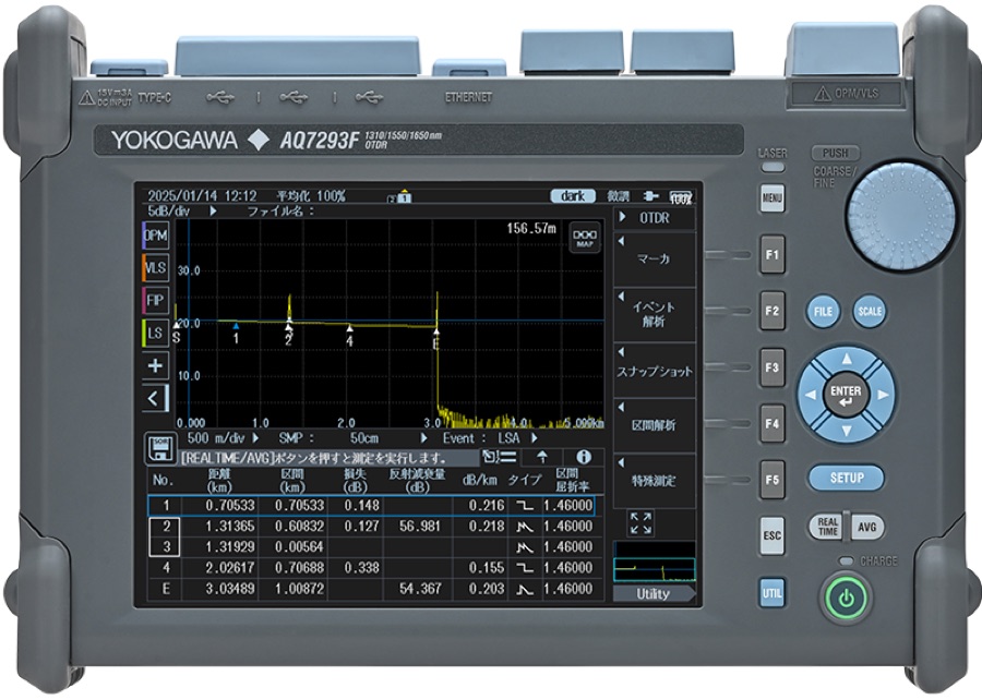
In practice: measure the link from end A, then from end B — necessarily with the same settings (wavelength, pulse, range), otherwise the average makes no sense. Modern reflectometers have built-in bidirectional analysis: you load both traces, the instrument matches the events and displays a table with the average loss of each — that is exactly the screen you see in the AQ7290 photo at the top of this page (a screenshot of bidirectional analysis, as in Fig. 38). The acceptance test report gets the averaged values.
The PON trace
In a point-to-multipoint network the test pulse splits in the splitter into all branches, and the backscatter returns from all of them at once and sums as a function of time. The trace from the OLT side is a superposition: steps where successive branches end, and reflections of the subscriber terminations — but you cannot tell which branch generates which event.
switch OLT ↔ ONT · enable APC and the termination reflections disappear (Fig. 42 vs 43)
Notice three things. First: with APC connectors at the subscribers the reflections disappear — what remains is the stepped sum of backscatter alone (Fig. 43). Second: measuring from the ONT side is incomparably more readable — a single path, a clear subscriber section and the splitter as a single big step (Fig. 44). That is why a subscriber link is serviced by measuring from the subscriber side. Third: beyond the splitter the subscriber sections lie close together, so a long pulse will resolve nothing there — an OTDR for PON needs high dynamic range precisely so it can get through the splitter with a short pulse. Dedicated FTTH designs combine short pulses of increased power with fast receiver recovery and high linearity.
Before you judge the result, check in the documentation which class loss budget the network operates in: each class (A…C+) defines the minimum and maximum allowed OLT–ONT path loss — e.g. the popular class B+ is the 13–28 dB window (Table 5). The sum of your steps and losses must fit within it; you will find the full class table in the cheat sheet.
On a live network the iron rule applies: measure only at the 1625/1650 nm maintenance wavelength, outside the transmission band (1310/1490 nm), with a filter protecting the reflectometer — the OLT signal reaches every termination non-stop, including the port you are plugging into, and can damage the instrument's photodetector. The filter must cut wavelengths below ~1610 nm with at least 40 dB of isolation — standard off-the-shelf CWDM/DWDM filters do not have enough. Modern reflectometers have a dedicated, filtered 1625 nm port; the most convenient designs detect line activity themselves before the measurement and enforce the maintenance wavelength.
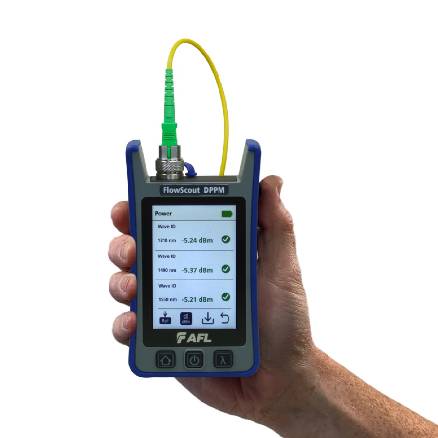
A live PON without guesswork: AFL FlowScout PON meters
On a working network the fastest diagnosis is a power measurement through the splitter: the FlowScout Downstream PON separates the 1490/1550 nm levels at the subscriber, and the Through-Mode version measures in-line, including 1310 nm upstream — without breaking the service.
See it in the INTERLAB catalog →When a PON goes down — the procedure step by step
Active equipment often reports the fault and its cause on its own — but when the system messages are not enough, craft takes over. The handbook closes the chapter with a decision diagram (Fig. 47). Walk through it live: make decisions like a dispatcher, and the procedure will lead you from symptom to repair.
* if the reflectometer has no 1625 nm port and the system does not use 1550 nm — the check measurement can be made at 1550 nm; when the line may be live, only through a live-network filter with at least 40 dB of isolation (a standard CWDM filter does not have enough)
Two things from this procedure are worth keeping in mind at all times. First, the order: power meter before reflectometer — a 1490 nm power measurement at the subscriber narrows the diagnosis to one of three paths within seconds. Second, instrument safety: on a live network you connect the reflectometer only through a filter — the OLT signal reaches every termination without pause. Modern designs, like AFL FlexScans with TestSafe technology, check line activity themselves before measuring and protect the photodetector — the handbook mentions this solution by name (section 5.5.3).
Build your own link
Drag blocks from the palette onto the fiber — the trace below recomputes live. Slide blocks along the strip, click a block to change its parameters, drag it off the strip to delete it. The red block is the fiber end — you can move it too.
hover over the chart = measure · scroll wheel = zoom · drag background = pan view
Try the PON classic: drag a splitter onto the fiber, set the split ratio to 1×8 (click the block) and shorten the pulse to 10 ns — the signal beyond the splitter drowns in the noise, because the dynamic range runs out. Lengthen the pulse: the signal climbs out of the noise, but the dead zones grow. This is exactly the trade-off a field technician wrestles with.
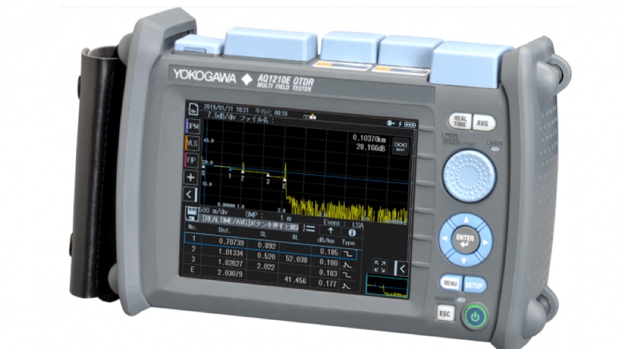 Yokogawa AQ1210
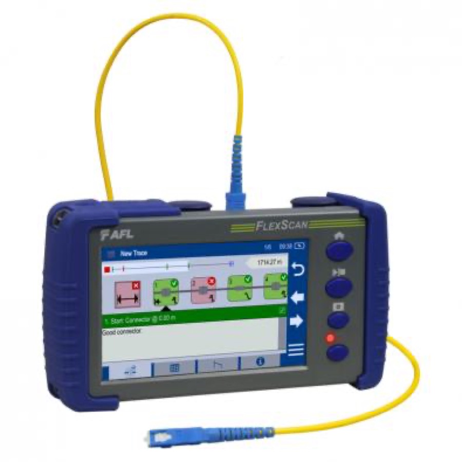 AFL FlexScan FS300
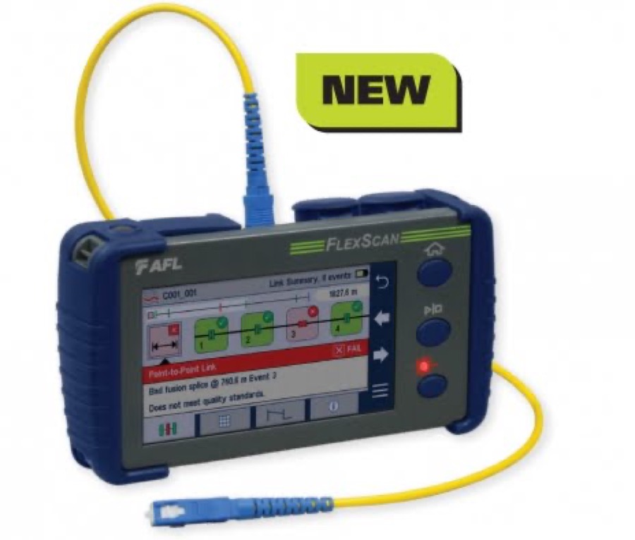 AFL FlexScan FS200
You have built a link, worked through gainers and PON — that is the end of the Academy's longest chapter. The good practices that protect these measurements are in chapter 6.